The IsoSurface plot-item lets you plot a 3D surface contour of zone data (e.g., displacement, velocity, pore pressure, temperature, stress, etc.) for a specified value (e.g., 0.25 m). By adding multiple IsoSurface plot-items of different values to your plot, you can build up visual representation of the spatial distribution of zone data, which may be easier to visualize than using a series of 2D slices. This tutorial will walk you through the work flow to start using this data analysis tool.
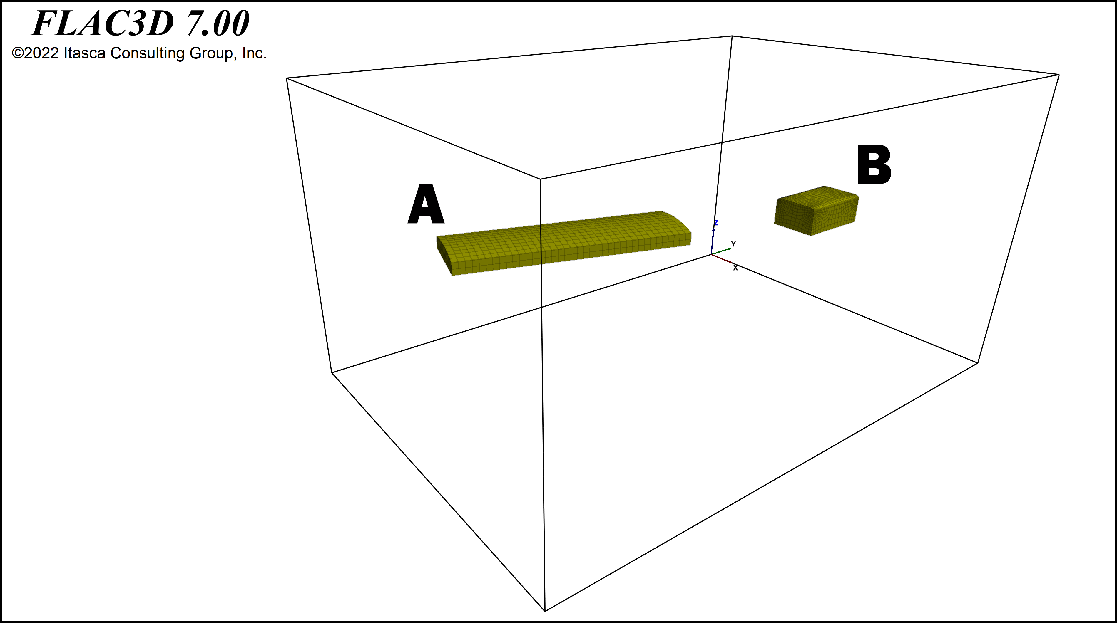
In this example, we will use a FLAC3D grid file, which was generated using the Itasca Griddle plug-in Rhino3D CAD software. The model contains two different underground caverns (different shapes, sizes, and orientation) within a region 475 ft long, 325 ft wide, and 250 ft high (Figure 1). The model uses the Zone Relax command to gradually excavate the first cavern (A) followed by the second (B). You can download the FLAC3D 7 project as a zipped bundle file below.
MODEL FILES (FLAC3D 7 | *.ZIP | 13.1 MB)
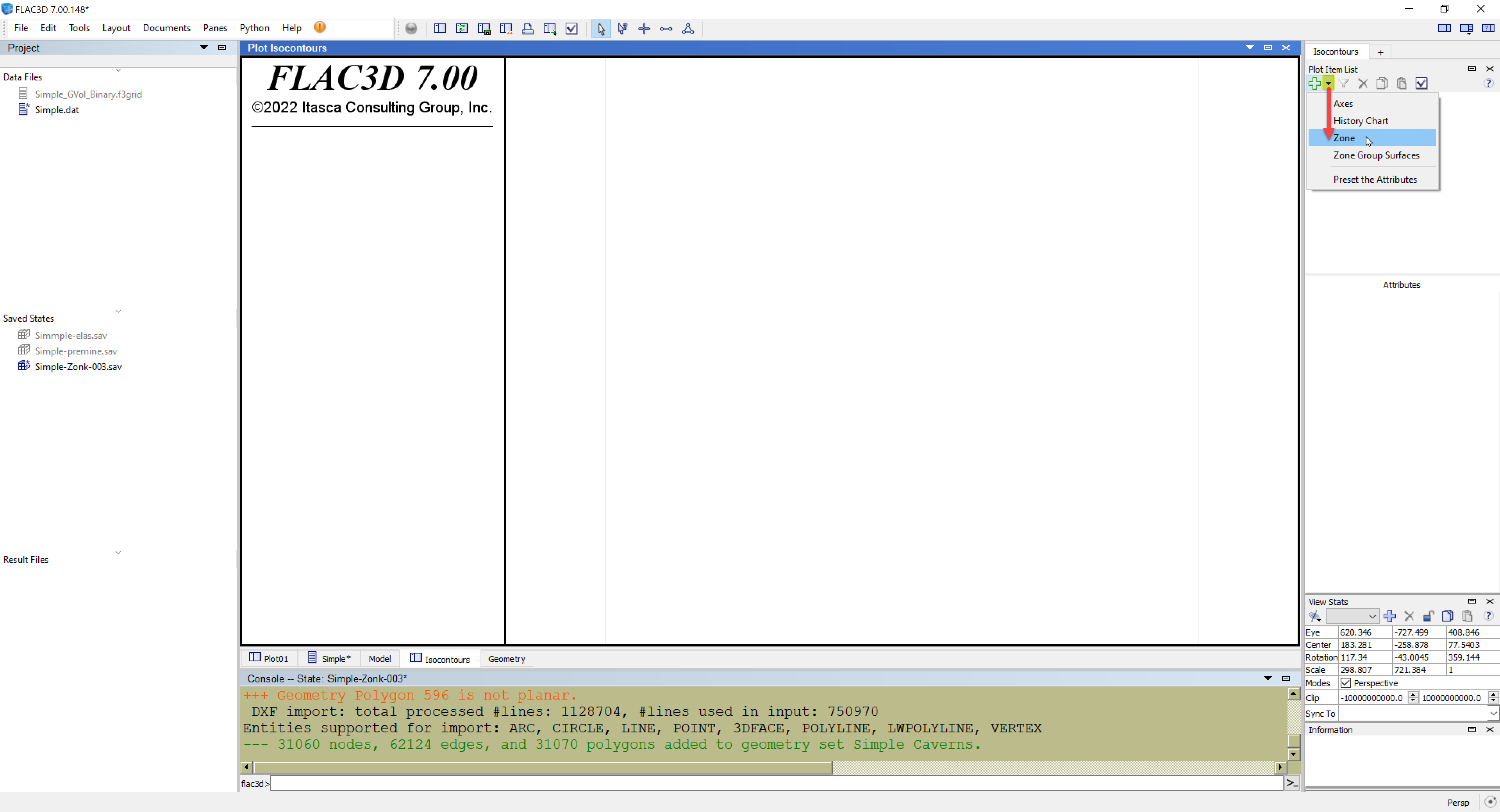
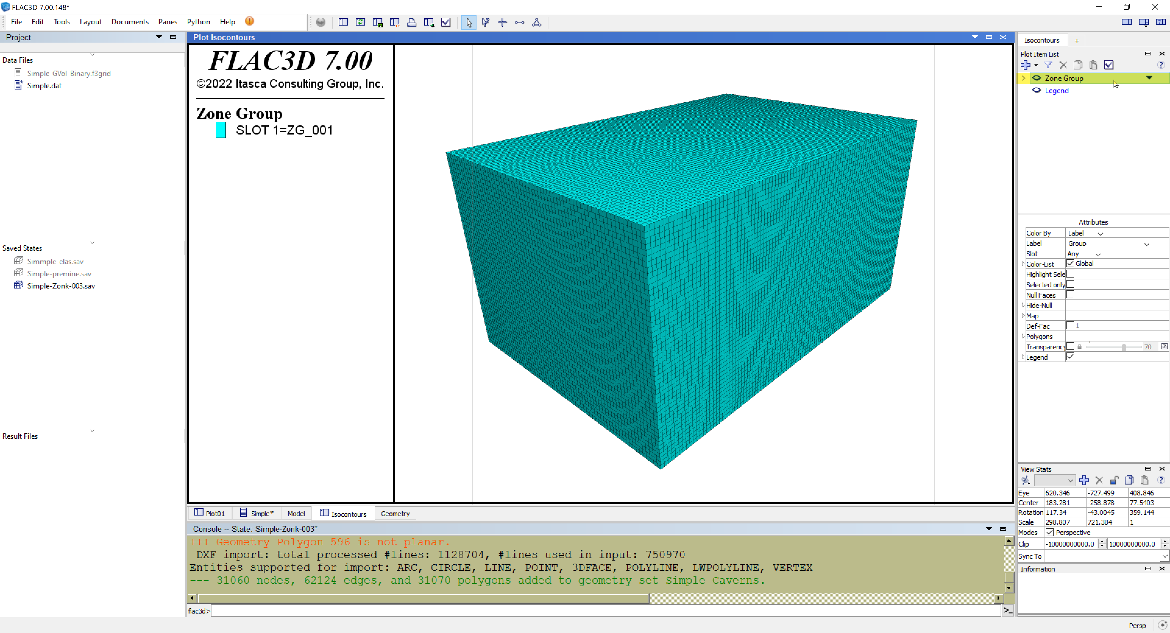
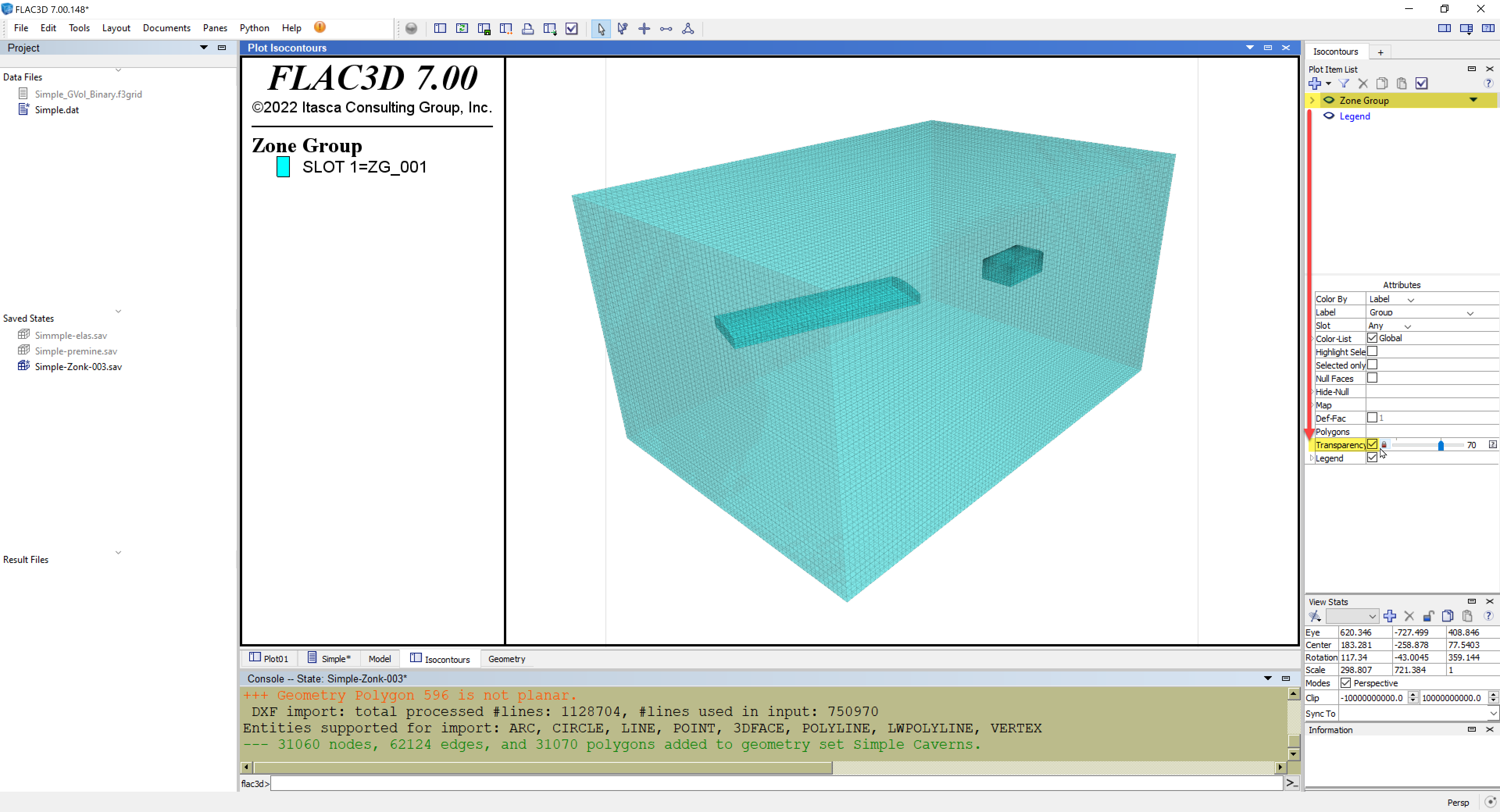
(1) Once you have unpackaged the tutorial files and run the model, or have restored one of your own models, let's plot the model zones as shown in Figure 2. The model zones should now be displayed (Figure 3). With the Zone Group plot-item selected, click its Transparency attribute to make the zones transparent. Now you can see both the external and the internal boundaries of the excavated caverns (Figure 4).
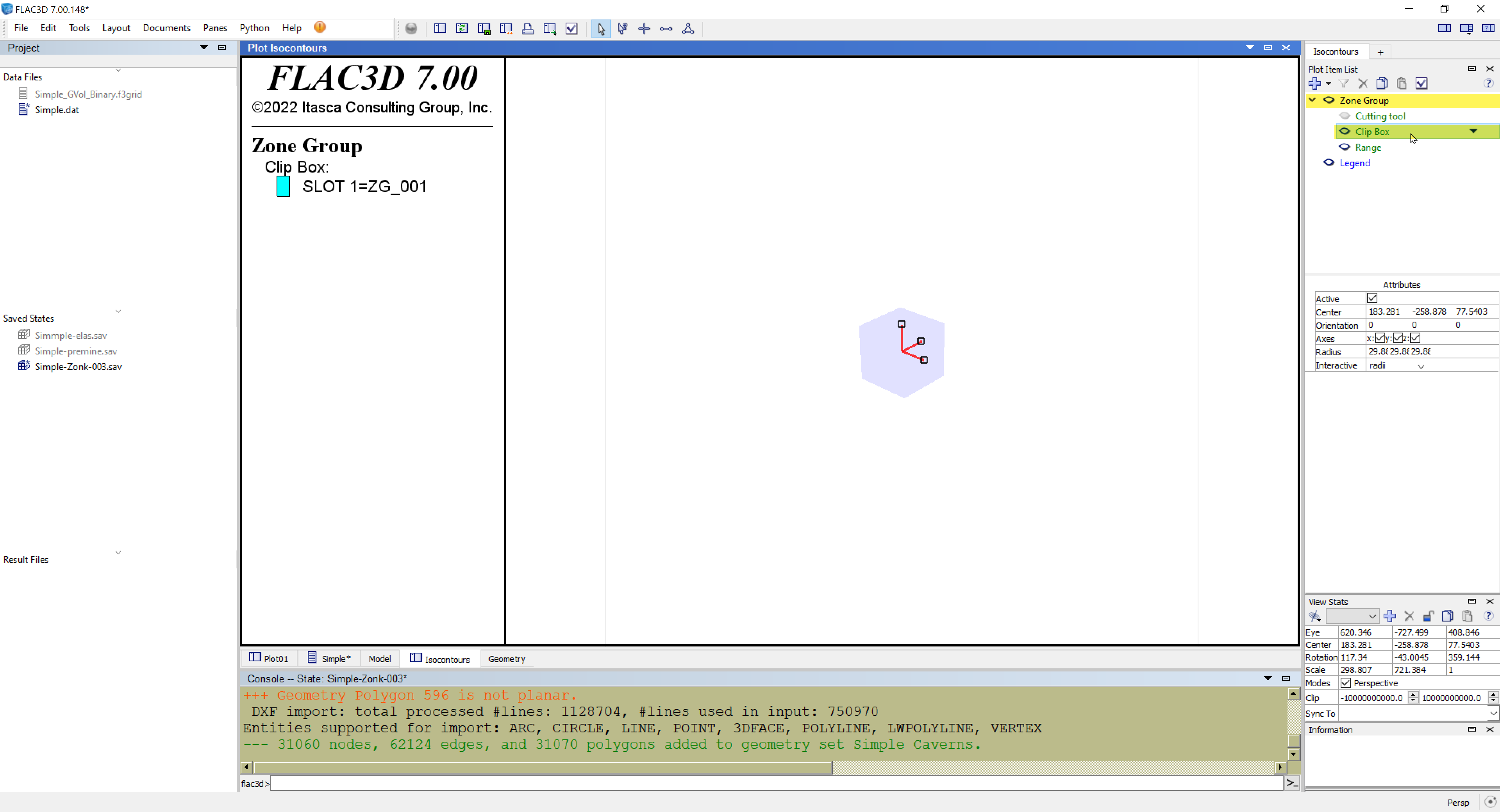
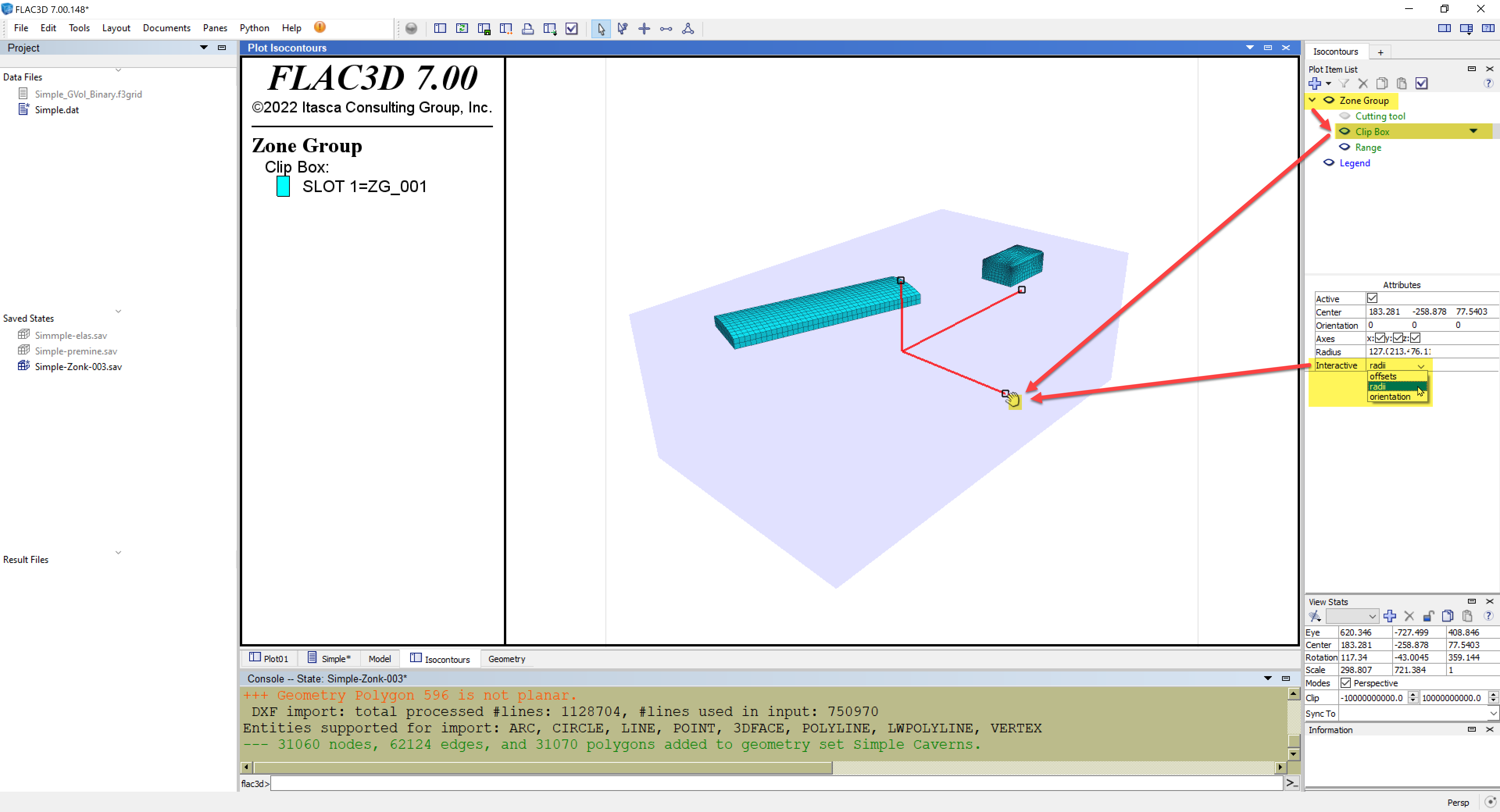
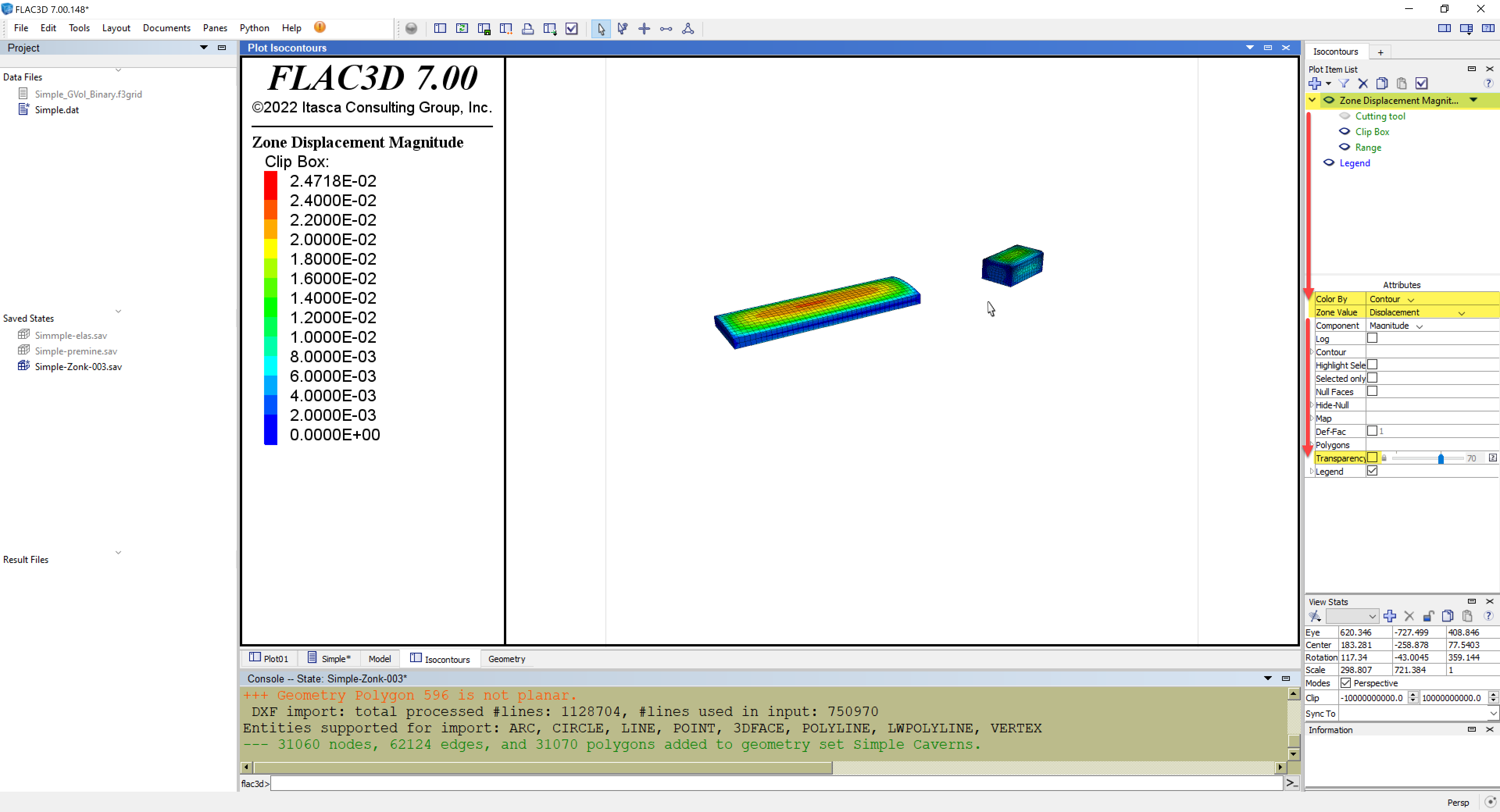
(2) Before we move on with IsoSurfaces, another useful way to view excavated regions in your model is via the Clip Box tool. You can find this by expanding the Zone Group plot-item. Click on the Clip Box eye icon to make it visible in the plot (Figure 5). You can grab the hand cursor and adjust the Clip Box radii, offsets, and orientation (toggle between these interactive modes under the Clip Box attributes) until the caverns become visible while excluding the exterior boundaries (Figure 6). As shown in Figure 7, you can change the Zone Group plot-item attributes to display total displacements on the cavern surfaces by coloring the plot-item by zone displacement value contours (rather than group labels); be sure to toggle off its Transparency for better viewing.
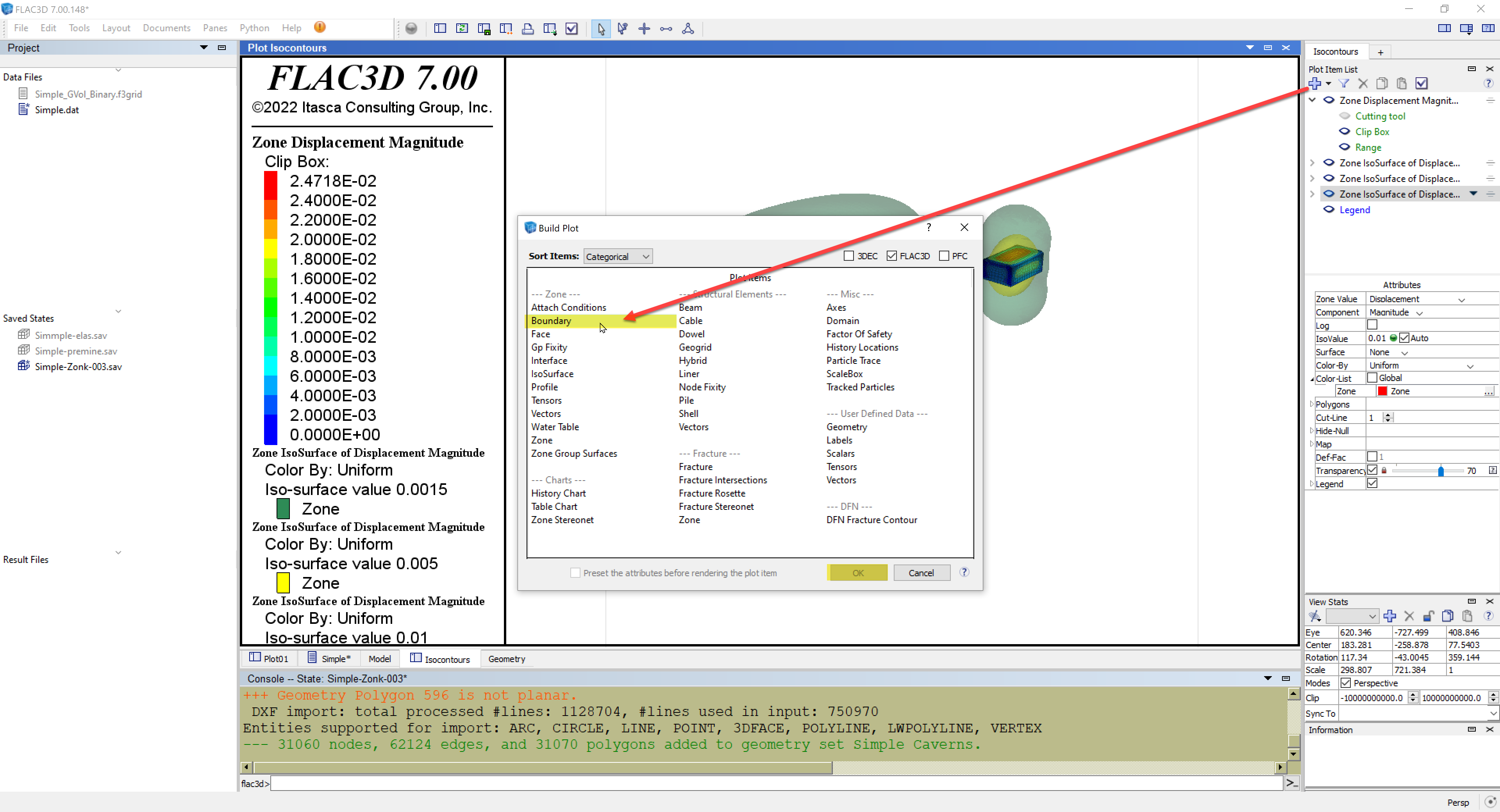
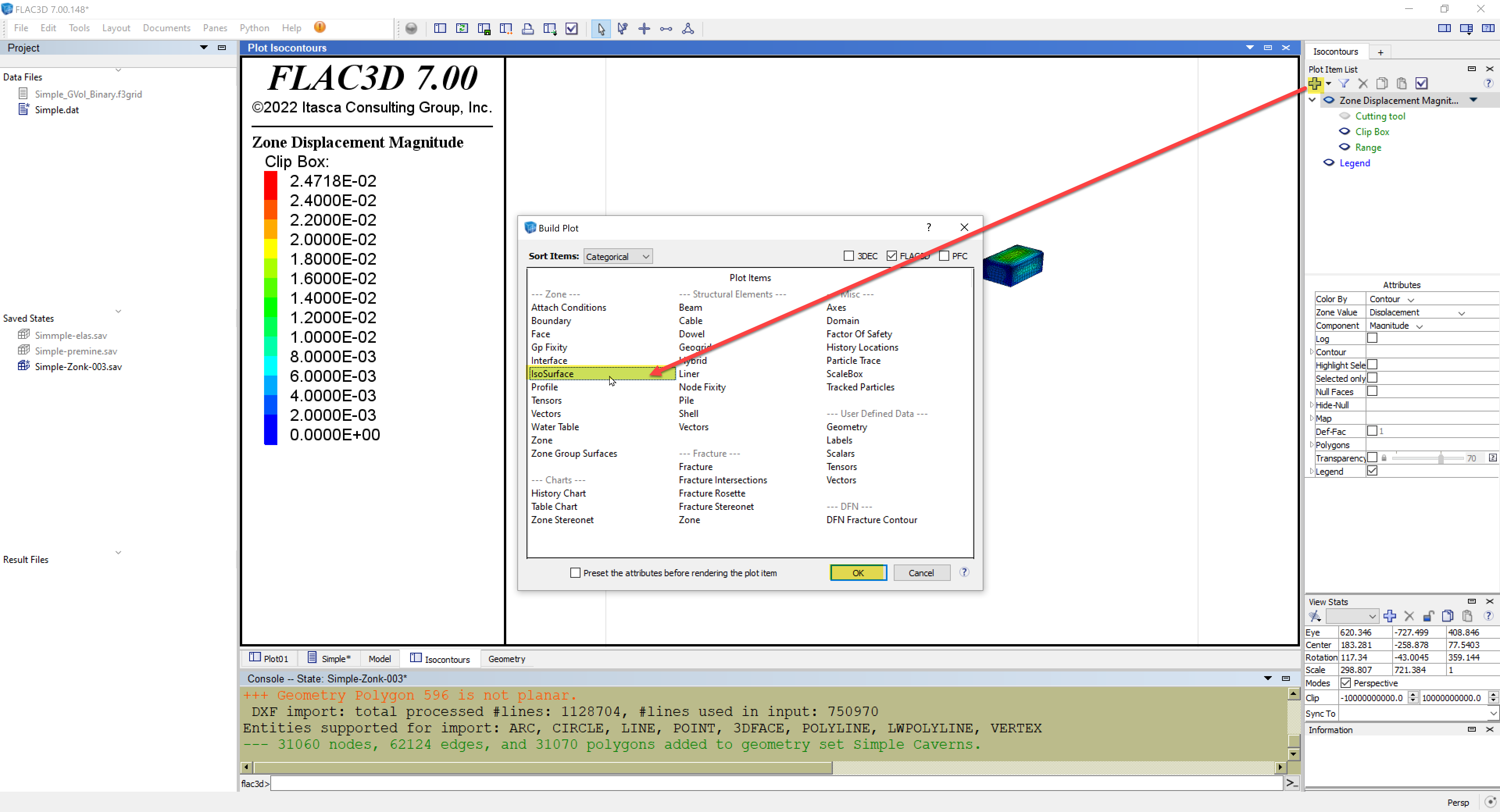
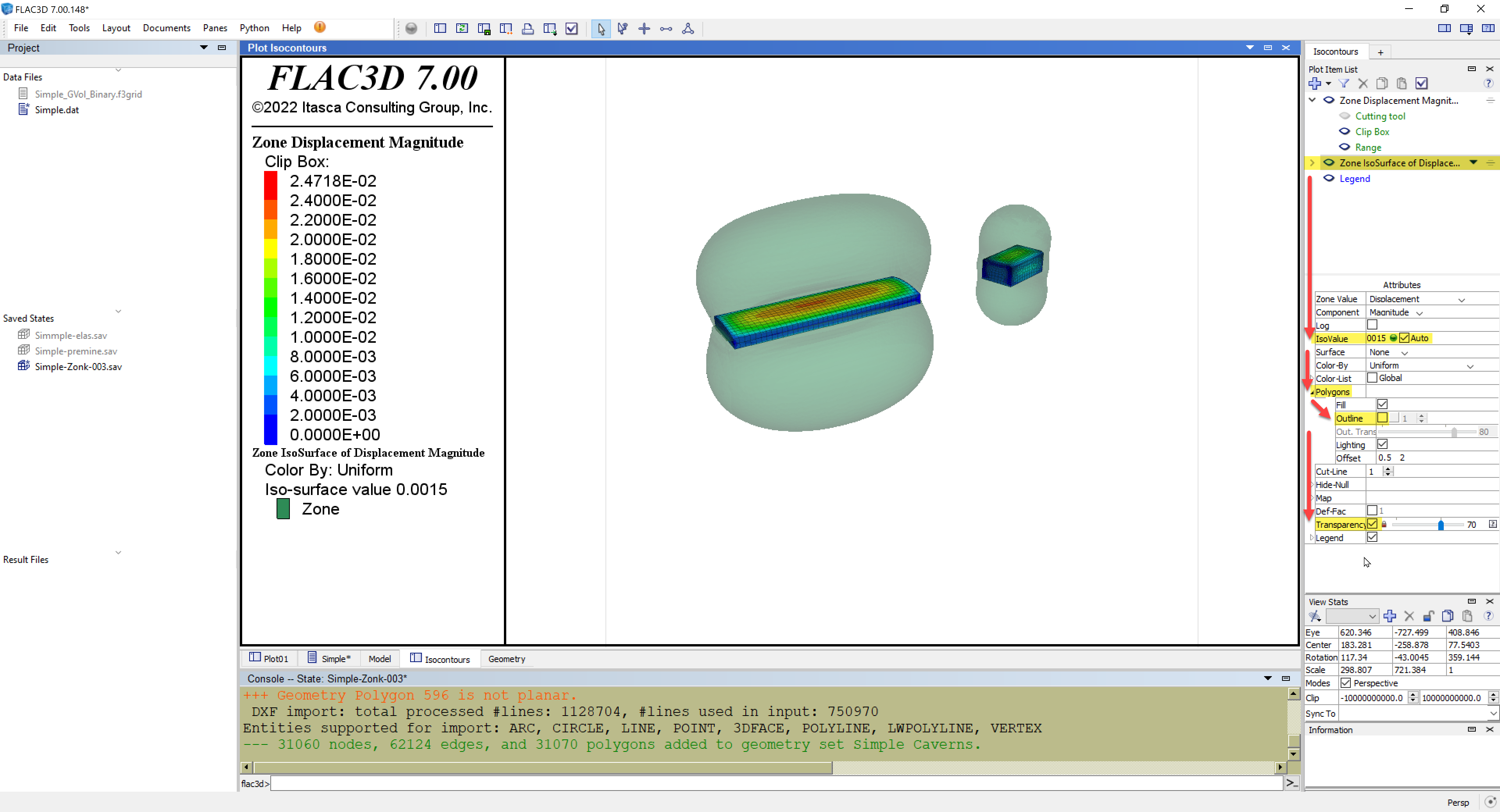
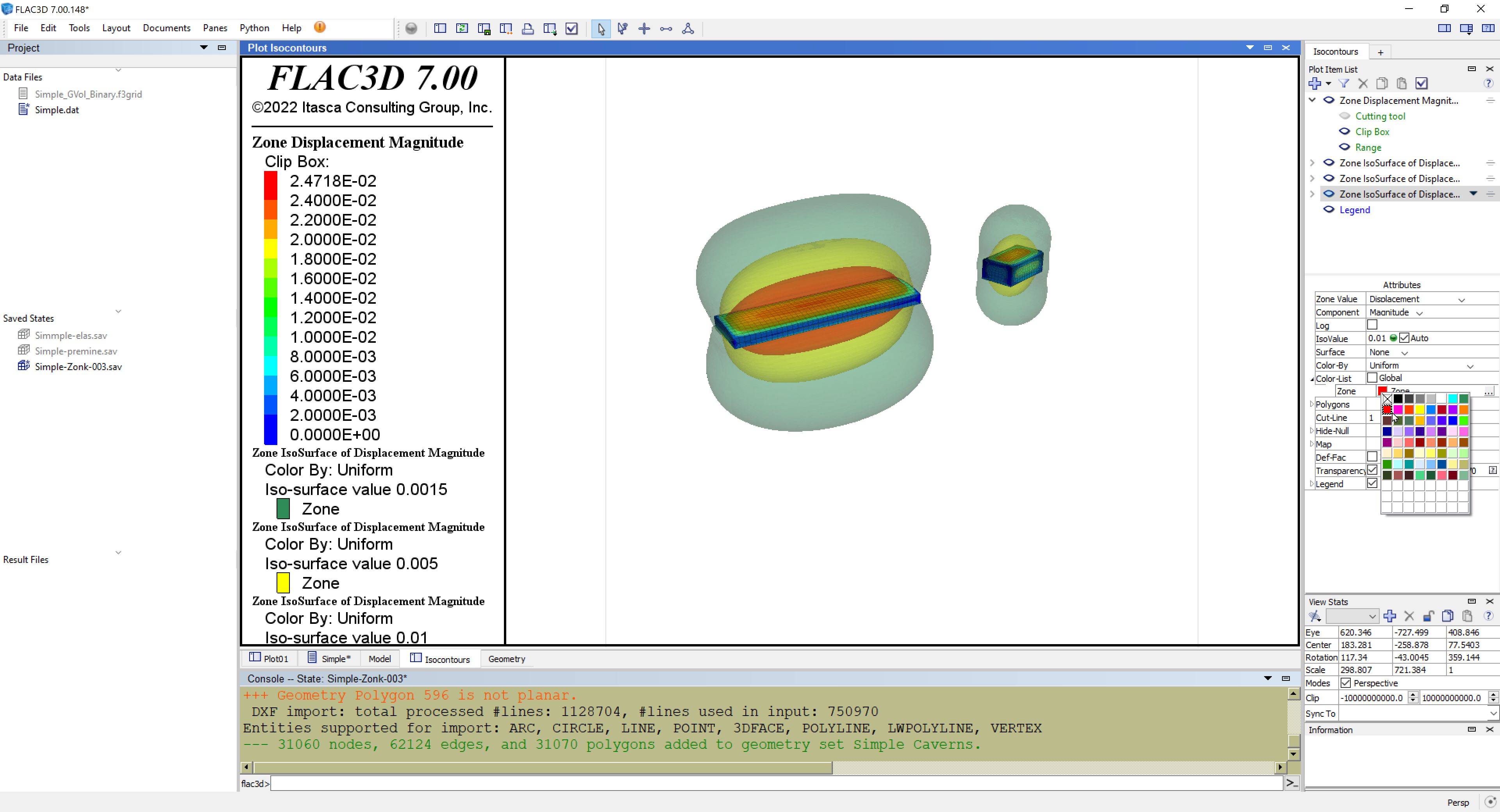
(3) Returning back to IsoSurfaces, add one of these plot-items as shown in Figure 8. Referring to Figure 9, select the Zone IsoSurface plot-item, select and specify 0.0015 as the value for the IsoSurface. You should now see a large, somewhat symmetrical ellipsoidal regions above and below both caverns. To match what's displayed in Figure 9 and make it easier to view along with the caverns, disable its Polygon Outline attribute and make the Zone IsoSurface plot-item transparent. Now add two more IsoSurface plot-items as above, but using values of 0.005 and 0.01, assigning different colors to each as shown in Figure 10.
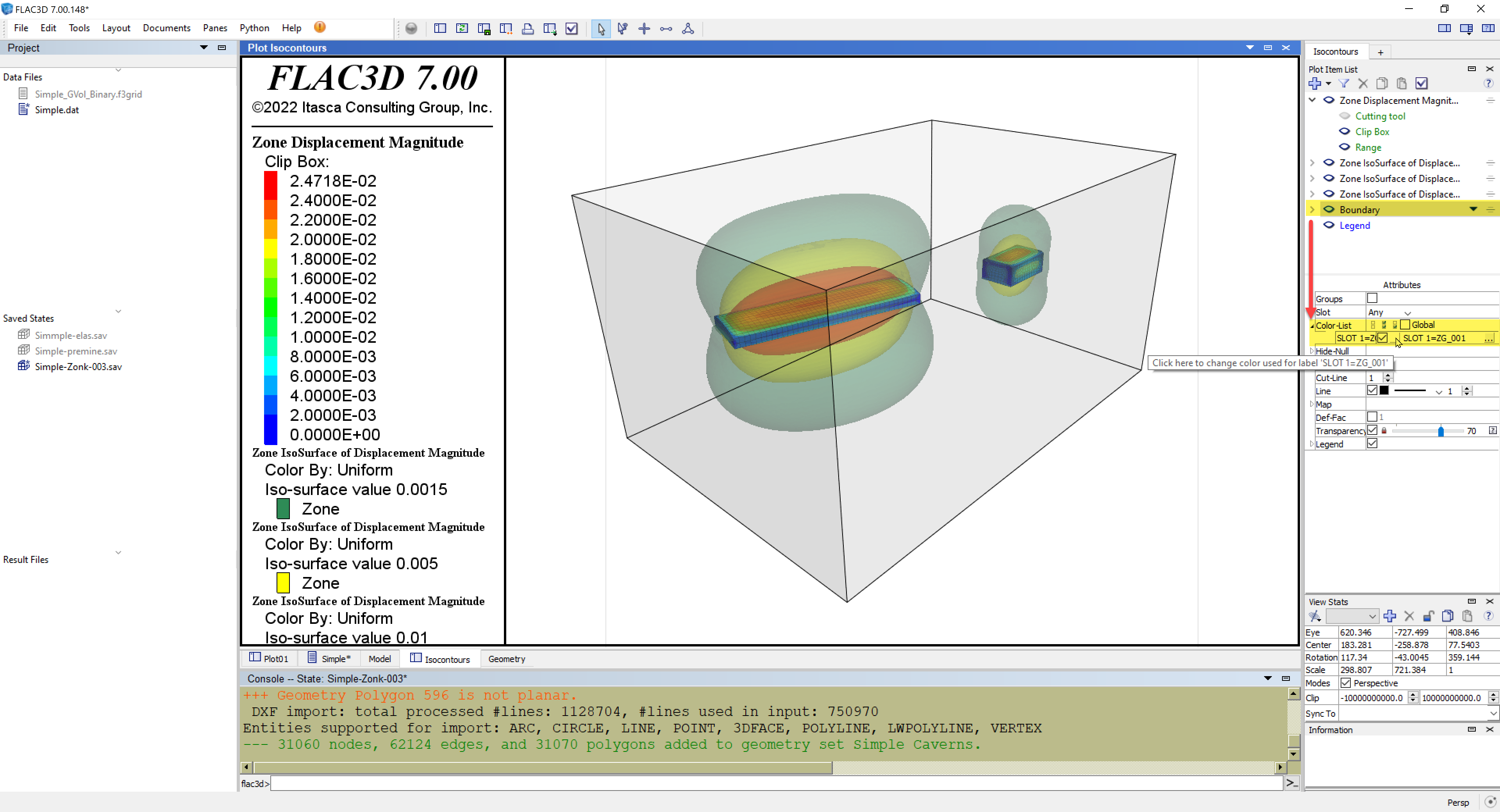
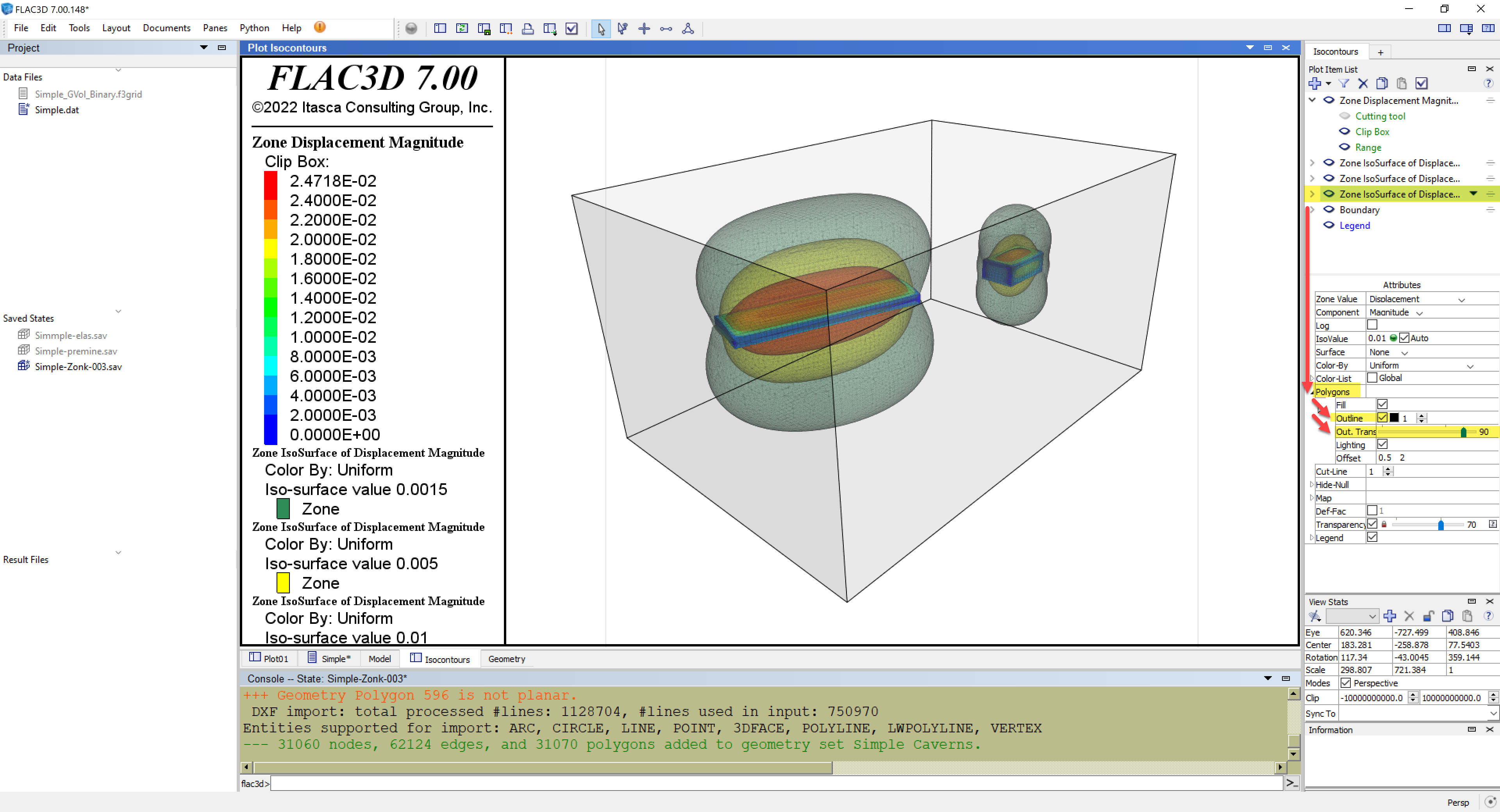
(4) To help provide some perspective, the Boundary plot-it in FLAC3D can be added (Figure 11) to provide a useful outline of the model boundaries as shown in Figure 12. An alternative way to render the IsoSurfaces is to enable their Polygons attributes but to increase their Transparency to 90%, which provides some shading while not obfuscating the other plot-items (Figure 13).